Alternative formulae for the Transverse Mercator projection

Introduction

These notes describe an attempt to derive formulae for the Transverse Mercator projection that should be (a) somewhat simpler, for the same order of accuracy, than the Redfearn formulae [1, 2] used by the Ordnance Survey of Great Britain, and (b) capable of routine extension (perhaps with the help of computerized algebra) to higher orders of accuracy.

The formulae below, when applied to Great Britain, are similar in accuracy to the OS formulae if carried to the 6th order. If carried to the 12th order they agree with Karney’s GeographicLib [3] to a fraction of nanometre when applied to Great Britain. They seem, however, less accurate than Karney’s method when applied to a wider area.

Only formulae for coordinate conversion are given at present. Formulae for scale and convergence may be added later.

The method used here is not entirely original, as shown by the appendix to Deakin et al. [4]. The idea is to carry out the projection from the ellipsoid to the plane in two stages: (i) from the ellipsoid to an intermediate sphere, (ii) from the sphere to the plane. Part (ii) and its inverse can be done by simple closed formulae containing hyperbolic functions. The hard work lies in part (i).

Conformal mappings

Let S and Σ be surfaces (e.g. plane, surface of sphere). A differentiable mapping from S to Σ is called conformal iff it preserves the angle at which curves intersect, or (equivalently) iff the scale at any point is the same in all directions. Let (x,y) be rectangular coordinates in S such that at every point the scales in x and y are equal, i.e. if σ denotes distance in S then ∂σ/∂x=∂σ/∂y. Let (ξ,η) be similar coordinates in Σ. Then the mapping is conformal iff at every point it satisfies the Cauchy–Riemann conditions:

∂ξ /∂x=∂η/∂y, ∂ξ /∂y=−∂η/∂x.

Assuming that the mapping can be put into the form

ξ=f0(y)+xf1(y)+(x2/2!) f2(y)+(x3/3!) f3(y)+⋯

η=g0(y)+xg1(y)+(x2/2!) g2(y)+(x3/3!) g3(y)+⋯

the Cauchy–Riemann conditions are equivalent to

f1=g0(1),  g1=−f0(1) f2=−f0(2),  g2=−g0(2) f3=−g0(3),  g3=f0(3) f4=f0(4),  g4=g0(4) …

So writing f,g for f₀,g₀ we see that the mapping is conformal iff it is of the form

ξ=f (y)+xg(1)(y)−(x2/2!) f (2)(y)−(x3/3!)g(3)(y)+(x4/4!) f (4)(y)+⋯ η=g(y)−x f (1)(y)−(x2/2!)g(2)(y)+(x3/3!) f (3)(y)+(x4/4!)g(4)(y)−⋯

(1)

Transverse Mercator projection

This is considered a suitable projection for a region such as Britain or New Zealand that extends more N–S than E–W. The Earth is taken to be an ellipsoid generated by rotating an ellipse about its smaller axis. A central meridian of longitude is chosen for the region to be mapped (e.g. for Britain the Ordnance Survey has chosen 2° W). The transverse Mercator projection from the ellipsoid to the (x,y) plane is such that

• It is conformal.
• The central meridian is mapped to the y-axis.
• The scale is the same at all points on the central meridian.

If μ₁ and μ₂ are two such mappings then μ₁⁻¹μ₂ is a conformal mapping of the plane taking (0,y) to (0,my+n), where m and n are constants. In the notation of the preceding section, we must then have f (y)=0 and g(y)=my+n, so that (x,y) is sent to (mx,my+n). Hence the transverse Mercator projection defined above is unique up to a change of scale and a shift parallel to the y-axis.

Notation

Where lower-case and upper-case of the same letter are given, lower-case refers to the ellipsoid and upper-case refers to the intermediate sphere.

• a = semi-major axis of ellipsoid
• b = semi-minor axis of ellipsoid
• e = eccentricity of ellipsoid; e²=(a²−b²)/a²
• ε=e²/(1−e²)=(a²−b²)/b²
• λ = longitude east of Greenwich meridian
• λ₀=λ for central meridian of projection (e.g. OS uses λ₀=−2°)
• ω,Ω = geographical longitude, relative to central meridian
• φ,Φ = geographical latitude
• ψ,Ψ = isometric latitude
• φ_m = fixed geographical latitude chosen by user, typically near mid-latitude of region of interest
• Φ_m,ψ_m,Ψ_m = values of Φ,ψ,Ψ corresponding to φ_m
• c=cosφ_m
• s=sinφ_m
• R = radius of intermediate sphere
• ρ = radius of curvature in meridian of ellipsoid = a(1−e²)(1−e²sin²φ)^−3/2 = a(1+ε)^1/2(1+εcos²φ)^−3/2
• F₀ = constant scale on central meridian
• E_off ,N_off = offsets added to easting and northing in order to give values measured from a conventional “false origin”

Geographical latitude φ at a point P on the ellipsoid is defined to be the angle between the normal at P and the plane of the equator. Isometric latitude ψ is defined in terms of φ by

ψ=tanh−1(sinφ)−e tanh−1(e sinφ).

(2)

It is straightforward to verify that if σ denotes distance on the ellipsoid then ∂σ/∂ω=∂σ/∂ψ at each point (ω,ψ). Hence the formulae for conformal mappings (first section) can be applied to the (ω,ψ) coordinate system.

Intermediate sphere

In the method of this web page, the transverse Mercator projection is split into two stages:

• (i) a conformal mapping from the ellipsoid to an intermediate sphere, taking the central meridian to the central meridian with constant scale;
• (ii) a transverse Mercator projection from the sphere to the (x,y) plane, taking the central meridian to the y-axis with unit scale.

From (2) with e=0 we get Ψ as the inverse Gudermann function of Φ, which can be written in three equivalent ways:

tanhΨ=sinΦ, sechΨ=cosΦ, sinhΨ=tanΦ.

Stage (ii) above (transverse Mercator from sphere to plane) is therefore given by simple closed formulae

tanh(x/R)=sechΨ sinΩ=cosΦ sinΩ tan(y/R)=sinhΨ secΩ=tanΦ secΩ,

(3)

whose equally simple inverse is given by (14) below.

We now need to work out stage (i), the projection from ellipsoid to sphere.

Outline of method

We are looking for a conformal mapping (1) with a change of notation: (Ω,Ψ) for (ξ,η), and (ω,ψ) for (x,y). Since the meridian ω=0 is projected to Ω=0, we have f=0, so that (1) becomes

Ω=ωg(1)(ψ)−(ω3/3!)g(3)(ψ)+(ω5/5!)g(5)(ψ)−⋯ Ψ=g(ψ)−(ω2/2!)g(2)(ψ)+(ω4/4!)g(4)(ψ)−⋯

(4)

The problem is to find g, and for this it suffices to consider the mapping of the central meridian, on which Ψ=g(ψ). Fix some geographical latitude φ_m near the centre of the region to be mapped (e.g. φ_m=55.6° is good for Britain) and let ψ_m,Φ_m,Ψ_m be the corresponding values of ψ,Φ,Ψ. Define δ=ψ−ψ_m.

To simplify the working and the result, we assume that on the central meridian (ω=0) Ψ is linear to third order in ψ around ψ_m, and write

Ψ|ω=0=g(ψ)=g(ψm+δ)=Ψm+Δ,

where

Δ=a1δ+a4δ4+a5δ5+a6δ6+⋯.

(5)

This is permissible because, as noted above, the projection has two degrees of freedom (scale and y-shift), so that we can choose it to make the terms in δ² and δ³ vanish. If for convenience we define a₀=Φ_m, a₂=a₃=0, then (4) and (5) can be developed as (cf. Deakin et al. [4], page 19)

Ψ+iΩ =g(ψ)+(iω)g(1)(ψ)+ (iω)2 g(2)(ψ)+ (iω)3 g(3)(ψ)+⋯ 2! 3! Ψ+iΩ =g(ψ+iω)=g(ψm+δ+iω) Ψ+iΩ = ∑ ∞ an(δ+iω)n= ∑ ∞ an ∑ n ( n ) δn−m(iω)m n=0 n=0 m=0 m Ψ+iΩ = ∑ ∞ ∑ ∞ (iω)m ( n ) anδn−m= ∑ ∞ ∑ ∞ (iω)m ( m+r ) am+rδr, m=0 n=m m m=0 r=0 m

(6)

from which Ψ and Ω can be found by equating real and imaginary parts.

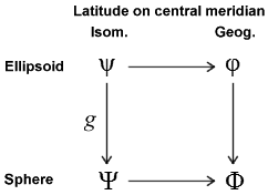
To find the coefficients a_n we will calculate Φ as a power series in δ in two ways, going via φ and Ψ respectively (see diagram). Equating coefficients of δⁿ will then give the result.

Details of method

φ from ψ. Recalling that δ=ψ−ψ_m, we express φ as a Taylor series in δ. We require the first few dⁿφ/dψⁿ. Differentiating (2) w.r.t. φ gives

dψ/dφ=(1−e2)/(1−e2sin2φ)cosφ=1/cosφ(1+εcos2φ)

whence

dφ/dψ =cosφ(1+εcos2φ) d2φ/dψ2 =−sinφcosφ(1+εcos2φ)(1+3εcos2φ) d3φ/dψ3 =cosφ(1+εcos2φ)[1−(2−12ε)cos2φ−(16ε−15ε2)cos4φ−18ε2cos6φ] d4φ/dψ4 =−sinφcosφ(1+εcos2φ)[1−(6−39ε)cos2φ−(90ε−135ε2)cos4φ−(238ε2+105ε3)cos6φ−162ε3cos8φ] …

This and similar lists below are to be extended, preferably with the aid of computerized algebra, up to the order of accuracy desired.

Φ from φ. If σ denotes distance along the central meridian then dσ/dφ=ρ=const×(1+εcos²φ)^−3/2. By hypothesis, the scale along the central meridian is constant, so that

Φ=p ∫ (1+εcos2φ)−3/2dφ+q,

(7)

where p and q are constants. The first few deriatives of Φ w.r.t. φ are therefore

dΦ/dφ =p(1+εcos2φ)−3/2 d2Φ/dφ2 =3pεsinφcosφ(1+εcos2φ)−5/2 d3Φ/dφ3 =3pε(1+εcos2φ)−7/2[−1+(2+4ε)cos2φ−3εcos4φ] d4Φ/dφ4 =3pε(1+εcos2φ)−9/2sinφcosφ[−(4+15ε)+(22ε+20ε2)cos2φ−9ε2cos4φ] d5Φ/dφ5 =3pε(1+εcos2φ)−11/2[(4+15ε) −(8+128ε+180ε2)cos2φ +(116ε+362ε2+120ε3)cos4φ −(164ε2+136ε3)cos6φ +27ε3cos8φ], …

Φ from ψ via φ. Using the above, express Φ as a Taylor series in φ−φ_m, and substitute for φ−φ_m a Taylor series in δ (=ψ−ψ_m). Setting c=cosφ_m,s=sinφ_m, we find after a routine calculation

Φ= Φm+rc(1+εc2)−1/2δ −(δ2/2!)s +(δ3/3!)(1−2c2−εc4) −(δ4/4!)s(1−6c2−9εc4−4ε2c6) +(δ5/5!)[1−20c2+(24−58ε)c4 +(72ε−64ε2)c6 +(77ε2−24ε3)c8 +28ε3c10] +⋯.

(8)

Φ from ψ via Ψ. The first few derivatives of Φ w.r.t. Ψ, written in terms of Φ, are

dΦ/dΨ =cosΦ, d2Φ/dΨ2 =−sinΦcosΦ, d3Φ/dΨ3 =cosΦ−2cos3Φ, d4Φ/dΨ4 =−sinΦ(cosΦ−6cos3Φ), d5Φ/dΨ5 =cosΦ−20cos3Φ+24cos5Φ.

So from (5) we get

Φ=Φm +δa1cosΦm −(δ2/2!)a12sinΦmcosΦm +(δ3/3!)a13(cosΦm−2cos3Φm)   +δ4[a4cosΦm −(1/4!)a14sinΦm(cosΦm−6cos3Φm)]   +δ5[a5cosΦm −a1a4sinΦmcosΦm +(1/5!)a15(cosΦm−20cos3Φm+24cos5Φm)   +⋯

(9)

On to the result. Equating coefficients of δ, δ², and δ³ in (8) and (9) gives respectively

a1cosΦm=rc(1+εc2)−1/2
a12sinΦmcosΦm=rsc(1+εc2)−1/2
a13(cosΦm−2cos3Φm)=rc(1−2c2−εc4)(1+εc2)−1/2

For a given φ_m these three equations are to be solved for Φ_rmm, p, and a₁. A straightforward calculation gives

tanΦm=tanφm(1+εcos2φm)−1/2	(10)
p=1+εcos2φm	(11)
a1=(1+εcos4φm)1/2.

To find a₄, note that

a1cosΦm=rc(1+εc2)−1/2=c(1+εc2)1/2, a1sinΦm=s

so that equating coefficients of δ⁴ in (5) and (9) and dividing by a₁cosΦ_m gives

−(1/4!)s(1−6c2−9εc4)=a4/a1−(1/4!)s[1+εc4−6c2(1+εc2)]

whence a₄=(1/6)a₁sεc⁴(1+εc²).

Similarly one calculates a₅,a₆,… as far as desired. This is probably not the best method for finding the a_i, as it is rather lengthy and does not explain why the factor (1+εc²) occurs in each a_i. However, with the help of computerized algebra it yields the following up to 12th order, where k=a₁εc⁴(1+εc²). Note that the factor s=sinφ_m appears in a_i for even but not odd i.

a4 = ks/6,

a5 = −(k/30)[(5 − 6c2) + εc2(6 − 7c2)],

a6 = (ks/180)[(23 − 39c2) + εc2(66 − 104c2) + ε2c4(48 − 70c2)],

a7 = −(k/1 260)[ (97 − 366c2 + 285c4)     + εc2 (534 − 1 834c2 + 1 354c4)     + ε2c4 (912 − 2 826c2 + 1 974c4)     + ε3c6 (480 − 1 368c2 + 910c4)],

a8 = (ks/10 080)[ (399 − 2 259c2 + 2 340c4)     + εc2 (3 786 − 18 201c2 + 17 091c4)     + ε2c4 (11 568 − 47 664c2 + 41 176c4)     + ε3c6 (13 920 − 50 832c2 + 40 964c4)     + ε4c8 (5 760 − 19 152c2 + 14 560c4)],

a9 = −(k/90 720)[ (1 617 − 15 822c2 + 35 145c4 − 21 420c6)     + εc2 (25 110 − 197 721c2 + 390 216c4 − 220 761c6)     + ε2c4 (122 832 − 810 108c2 + 1 456 888c4 − 777 368c6)     + ε3c6 (254 880 − 1 476 432c2 + 2 465 576c4 − 1 253 156c6)     + ε4c8 (236 160 − 1 240 992c2 + 1 951 360c4 − 951 748c6)     + ε5c10 (80 640 − 392 832c2 + 587 664c4 − 276 640c6)],

a10 = (ks/907 200)[ (6 511 − 96 003c2 + 284 580c4 − 216 720c6)     + εc2 (160 362 − 1 741 062c2 + 4 357 044c4 − 2 979 576c6)     + ε2c4 (1 183 536 − 10 218 210c2 + 22 614 831c4 − 14 293 933c6)     + ε3c6 (3 777 120 − 27 694 080c2 + 55 715 568c4 − 33 050 400c6)     + ε4c8 (5 892 480 − 38 260 512c2 + 71 319 600c4 − 40 132 128c6)     + ε5c10 (4 435 200 − 26 210 304c2 + 45 899 424c4 − 24 698 800c6)     + ε6c12 (1 290 240 − 7 070 976c2 + 11 753 280c4 − 6 086 080c6)],

a11 = −(k/9 979 200)[ (26 129 − 612 942c2 + 2 973 465c4 − 4 769 100c6 + 2 404 080c8)     + εc2 (1 001 238 − 16 079 440c2 + 64 079 286c4 − 91 147 284c6 + 42 371 064c8)     + ε2c4 (10 751 184 − 133 032 942c2 + 462 342 495c4 − 603 358 772c6 + 264 215 043c8)     + ε3c6 (49 606 560 − 513 290 016c2 + 1 608 671 808c4 − 1 961 068 704c6 + 818 045 920c8)     + ε4c8 (116 035 200 − 1 054 446 048c2 + 3 047 708 544c4 − 3 514 163 808c6 + 1 407 298 464c8)     + ε5c10 (144 587 520 − 1 190 221 056c2 + 3 223 093 824c4 − 3 547 726 976c6 + 1 372 021 728c8)     + ε6c12 (91 607 040 − 697 432 320c2 + 1 789 882 560c4 − 1 894 042 304c6 + 710 673 040c8)     + ε7c14 (23 224 320 − 165 934 080c2 + 407 062 656c4 − 416 391 360c6 + 152 152 000c8)],

a12 = (ks/119 750 400)[ (104 687 − 3 695 043c2 + 23 932 260c4 − 47 995 920c6 + 29 030 400c8)     + εc2 (6 164 202 − 134 900 843c2 + 679 980 393c4 − 1 168 763 544c6 + 636 663 600c8)     + ε2c4 (94 019 376 − 1 503 338 308c2 + 6 400 822 965c4 − 9 876 665 101c6 + 4 988 315 196c8)     + ε3c6 (603 577 440 − 7 805 457 864c2 + 29 310 906 258c4 − 41 588 254 065c6 + 19 773 581 543c8)     + ε4c8 (1 987 701 120 − 22 054 179 456c2 + 75 126 837 408c4 − 99 606 227 856c6 + 45 043 964 496c8)     + ε5c10 (3 648 718 080 − 36 037 592 064c2 + 113 548 973 184c4 − 142 326 334 672c6 + 61 685 211 984c8)     + ε6c12 (3 779 112 960 − 34 051 258 368c2 + 100 637 983 296c4 − 120 305 983 424c6 + 50 268 203 216c8)     + ε7c14 (2 066 964 480 − 17 285 068 800c2 + 48 419 217 792c4 − 55 579 694 016c6 + 22 494 311 840c8)     + ε8c16 (464 486 400 − 3 650 549 760c2 + 9 769 503 744c4 − 10 826 175 360c6 + 4 260 256 000c8)].

Radius of intermediate sphere

We chose above that the projection from intermediate sphere to plane should have unit scale on the central meridian. We therefore need to choose R (the radius of the intermediate sphere) so that the projection from ellipsoid to intermediate sphere has the required constant scale F₀ on the central meridian. It suffices to do this at the base latitude φ_m. If σ denotes distance along the central meridian, then at φ_m we have

dφ/dσ = ρ−1 = a−1(1 + ε)−1/2(1 + εc2)3/2

dΦ/dφ = p(1 + εc2)−3/2 = (1 + εc2)−1/2   from (7) and (11)

whence the scale on the central meridian is Ra⁻¹(1 + ε)^−1/2(1 + εc²). Equating this to F₀ gives

R = aF0(1 + ε)1/2(1 + εc2)−1.

(12)

Geographical to grid

The method for converting geographical coordinates (φ, ω) on the ellipsoid to grid coordinates (E, N) can now be given.

Find the isometric latitude ψ from (2), and set δ = ψ − ψ_m. Calculate R from (12) and calculate as many of a₁, a₄, a₅, … as desired.

Longitude and isometric latitude on the sphere can now be found from from (6). If we equate real and imaginary parts, and evaluate the binomial coefficients, this gives the following series for Ψ and Ω. Terms containing a_i beyond those calculated should be ignored.

Ψ = Ψm + a1δ + a4δ4 + a5δ5 + a6δ6 + a7δ7 + a8δ8 + a9δ9 + a10δ10 + a11δ11 + a12δ12 + …     − ω2(6a4δ2 + 10a5δ3 + 15a6δ4 + 21a7δ5 + 28a8δ6 + 36a9δ7 + 45a10δ8 + 55a11δ9 + 66a12δ10 + …)     + ω4(a4 + 5a5δ + 15a6δ2 + 35a7δ3 + 70a8δ4 + 126a9δ5 + 210a10δ6 + 330a11δ7 + 495a12δ8 + …)     − ω6(a6 + 7a7δ + 28a8δ2 + 84a9δ3 + 210a10δ4 + 462a11δ5 + 924a12δ6 + …)     + ω8(a8 + 9a9δ + 45a10δ2 + 165a11δ3 + 495a12δ4 + …)     − ω10(a10 + 11a11δ + 66a12δ2 + …)     + ω12(a12 + …)     − … Ω = ω(a1 + 4a4δ3 + 5a5δ4 + 6a6δ5 + 7a7δ6 + 8a8δ7 + 9a9δ8 + 10a10δ9 + 11a11δ10 + 12a12δ11 + …     − ω3(4a4δ + 10a5δ2 + 20a6δ3 + 35a7δ4 + 56a8δ5 + 84a9δ6 + 120a10δ7 + 165a11δ8 + 220a12δ9 + …)     + ω5(a5 + 6a6δ + 21a7δ2 + 56a8δ3 + 126a9δ4 + 252a10δ5 + 462a11δ6 + 792a12δ7 + …)     − ω7(a7 + 8a8δ + 36a9δ2 + 120a10δ3 + 330a11δ4 + 792a12δ5 + …)     + ω9(a9 + 10a10δ + 55a11δ2 + 210a12δ3 + …)     − ω11(a11 + 12a12δ + …)     + …

(13)

Having found Ψ and Ω, calculate the grid coordinates as

E = R tanh−1(sinΩ/coshΨ) + Eoff ,

N = R tan−1(sinhΨ/cosΩ) + Noff .

It remains to find the constant offsets E_off and N_off. There is no difficulty with E_off, which is simply the conventional easting of points on the central meridian (e.g. for Great Britain the OS uses E_off = 400 000 m).

N_off is implicitly defined by choosing a point on the central meridian, say with latitude φ₀, and specifying its conventional northing, say N₀. (E.g. for Great Britain the OS chooses φ₀ = 49° and N₀ = −100000 m.) One could estimate N_off by feeding φ = φ₀ into the above procedure, but since φ₀ may be outside the region of greatest accuracy the following method is preferable.

Let N_m be the northing of the point on the central meridian with latitude φ_m, before applying the conventional offset. Let D be the distance along the central meridian measured northwards from φ₀ to φ_m, perhaps calculated by one of the methods for meridian arc suggested on this website. Then we require N_off = F₀D + N₀ − N_m. The value of N_m can be found from (10), whence

Noff = F0D + N0 − R tan−1((1 + εc2)−1/2tanφm).

Grid to geographical

The problem here is: Given grid coordinates E and N, find geographical latitude φ and longitude λ. It is a question of reversing the above-described method of finding grid from geographical coordinates.

Having found the constants E_off and N_off as above, define

x = E − Eoff ,   y = N − Noff .

The inverse of (3) above is given by

tanhΨ = sech(x/R)sin(y/R), tanΩ = sinh(x/R)sec(y/R),

(14)

from which we get the isometric latitude Ψ and longitude Ω on the intermediate sphere.

The projection from sphere to ellipsoid is analogous to the projection from ellipsoid to sphere. We first need to invert the power series (5), so as to get δ as a power series in Δ = Ψ − Ψ_m. The absence of terms in δ² and δ³ simplifies the result, which can be written

δ = b1Δ − b4Δ4 − b5Δ5 − b6Δ6 − …,

where up to 12th order

b1 = 1 / a1,

b4 = a4 / a15,

b5 = a5 / a16,

b6 = a6 / a17,

b7 = (a1a7 − 4a42) / a19,

b8 = (a1a8 − 9a4a5) / a110,

b9 = (a1a9 − 5a52 − 10a4a6) / a111,

b10 = (a12a10 − 11a1a5a6 − 11a1a4a7 + 22a43) / a113,

b11 = (a12a11 − 6a1a62 − 12a1a5a7 − 12a1a4a8 + 78a42a5) / a114,

b12 = (a12a12 − 13a1a6a7 − 13a1a5a8 − 13a1a4a9 + 91a4a52 + 91a42a6) / a115.

The reasoning that led to (13) above leads to exactly analogous formulae for the ellipsoid coordinates ψ and ω:

ψ = ψm + b1Δ + b4Δ4 + b5Δ5 + b6Δ6 + b7Δ7 + b8Δ8 + b9Δ9 + b10Δ10 + b11Δ11 + b12Δ12 + …     − Ω2(6b4Δ2 + 10b5Δ3 + 15b6Δ4 + 21b7Δ5 + 28b8Δ6 + 36b9Δ7 + 45b10Δ8 + 55b11Δ9 + 66b12Δ10 + …)     + Ω4(b4 + 5b5Δ + 15b6Δ2 + 35b7Δ3 + 70b8Δ4 + 126b9Δ5 + 210b10Δ6 + 330b11Δ7 + 495b12Δ8 + …)     − Ω6(b6 + 7b7Δ + 28b8Δ2 + 84b9Δ3 + 210b10Δ4 + 462b11Δ5 + 924b12Δ6 + …)     + Ω8(b8 + 9b9Δ + 45b10Δ2 + 165b11Δ3 + 495b12Δ4 + …)     − Ω10(b10 + 11b11Δ + 66b12Δ2 + …)     + Ω12(b12 + …)     − … ω = Ω(b1 + 4b4Δ3 + 5b5Δ4 + 6b6Δ5 + 7b7Δ6 + 8b8Δ7 + 9b9Δ8 + 10b10Δ9 + 11b11Δ10 + 12b12Δ11 + …     − Ω3(4b4Δ + 10b5Δ2 + 20b6Δ3 + 35b7Δ4 + 56b8Δ5 + 84b9Δ6 + 120b10Δ7 + 165b11Δ8 + 220b12Δ9 + …)     + Ω5(b5 + 6b6Δ + 21b7Δ2 + 56b8Δ3 + 126b9Δ4 + 252b10Δ5 + 462b11Δ6 + 792b12Δ7 + …)     − Ω7(b7 + 8b8Δ + 36b9Δ2 + 120b10Δ3 + 330b11Δ4 + 792b12Δ5 + …)     + Ω9(b9 + 10b10Δ + 55b11Δ2 + 210b12Δ3 + …)     − Ω11(b11 + 12b12Δ + …)     + …

The isometric latitude ψ on the ellipsoid needs to be converted to geographical latitude φ by inverting equation (2). This can be done by iteration or one of the other methods for isometric to geographic latitude suggested on this website.

Finally the longitude λ with respect to Greenwich is given by λ = λ₀ + ω.

Michael Behrend, October 2011

 

References

[1] Ordnance Survey (UK), A guide to coordinate systems in Great Britain. Downloaded 2011-09-09 from
http://www.ordnancesurvey.co.uk/oswebsite/gps/docs/A_Guide_to_Coordinate_Systems_in_Great_Britain.pdf
2015-09-24 Now at https://www.ordnancesurvey.co.uk/docs/support/guide-coordinate-systems-great-britain.pdf

[2] https://en.wikipedia.org/wiki/Transverse_Mercator:_Redfearn_series

[3] C.F.F. Karney, GeographicLib. Available from http://geographiclib.sourceforge.net

[4] R.E. Deakin, M.N. Hunter, & C.F.F. Karney, “The Gauss–Krüger projection”. Presented at the Victoria Regional Survey Conference, Warrnambool, 10–12 September 2010. Downloaded 2011-08-30 from
http://user.gs.rmit.edu.au/rod/files/publications/Gauss-Krueger%20Warrnambool%20Conference.pdf
2015-09-24 Now at http://www.mygeodesy.id.au/documents/Gauss-Krueger%20Warrnambool%20Conference.pdf