Converting isometric latitude to geographic latitude

If the Earth is modelled as an oblate spheroid with eccentricity e, then the isometric latitude ψ is defined in terms of the geographic latitude φ by

ψ = tanh−1(sinφ) − e tanh−1(e sinφ).

(1)

The problem is to invert (1) and find φ when ψ is given. We do this here by finding sinφ. For other approaches, see e.g. Wolfram MathWorld [1].

If we define s = sinφ then (1) becomes

ψ = tanh−1(s) − e tanh−1(es),

(2)

and we require s given ψ. Three methods are briefly described below.

Method 1: Iteration

This is straightforward. Starting with s₀ = tanh ψ, or better s₀ = tanh ψ / (1 − e²), we iterate

sn+1 = tanh(ψ + e tanh−1(esn))

until the desired accuracy has been achieved.

Method 2: Power series obtained by iteration

Write t = tanh ψ. From (2)

ψ = tanh−1(s) − e2s − e4s3/3 − e6s5/5 − …

whence

s = tanh(ψ + e2s + e4s3/3 + e6s5/5 + …).

Substituting the first approximation s = t in the RHS gives

s = tanh(ψ + e2t) + O(e4) = (1 + e2)t − e2t3 + O(e4).

Substituting the second approximation s = (1 + e²)t − e²t³ gives a third approximation with error O(e⁶), and so on. Taking the approximation up to terms in e¹², with error O(e¹⁴), we find

sinφ = F1(e)t − F3(e)t3 + F5(e)t5 − F7(e)t7 + F9(e)t9 − F11(e)t11 + F13(e)t13 − …

where

F1(e) = 1 + e2 + e4 + e6 + e8 + e10 + e12 + … F3(e) = e2 + (8/3)e4 + 5e6 + 8e8 + (35/3)e10 + 16e12 + … F5(e) = (5/3)e4 + (36/5)e6 + (293/15)e8 + (127/3)e10 + 80e12 + … F7(e) = (16/5)e6 + (6 017/315)e8 + (21 319/315)e10 + (58 111/315)e12 + … F9(e) = (2 069/315)e8 + (1 751/35)e10 + (619 831/2 835)e12 + … F11(e) = (883/63)e10 + (2 892 031/22 275)e12 + … F13(e) = (1 594 444/51 975)e12 + …   ….

It may be more convenient to rearrange this as a power series in e². Method 2 thus becomes:

sinφ = t + e2 t (1 − t2)[1 + G1(t)e2 + G2(t)e4 + G3(t)e6 + …]

where

G1(t) = 1 − (5/3)t2, G2(t) = 1 − 4t2 + (16/5)t4, G3(t) = 1 − 7t2 + (188/15)t4 − (2069/315)t6, G4(t) = 1 − (32/3)t2 + (95/3)t4 − (11 344/315)t6 + (883/63)t8, G5(t) = 1 − 15t2 + 65t4 − (37 636/315)t6 + (281 107/2 835)t8 − (1 594 444/51 975)t10,   ….

2016-10-22 Corrected the following errors.
The coefficient 16/5 in F₇ was mistyped as16/15.
The coefficient 188/15 in G₃ appeared as 1316/105 (correct value, but not in its lowest terms).

Method 3: Another power series method

If we define ε = e ² / (1 − e ²), then up to O(e¹⁴) the first two F’s in the preceding method are given by

F1(e) = 1 + ε,      F3(e) = (1 + ε)(3 + 2ε)ε/3.

In fact these expressions are exact, and all the F’s are finite polynomials in ε. To see this, note that (2) gives

d s = (1 − s2)(1 − e2s2) = (1 − s2)(1 + ε − ε s2) . d t (1 − e2)(1 − t2) (1 − t2)

Consequently, if we set

dn s = (1 − s2)(1 + ε − ε s2) ∑ c(n; i, j)sitj d tn (1 − t2)n

then after some routine calculation we find the recurrence

c(n + 1; i, j) = ε(i + 1)c(n; i − 3, j) − (i + 1)(1 + 2ε)c(n; i − 1, j) + (i + 1)(1 + ε)c(n; i + 1, j)     + (2n − j + 1)c(n; i, j − 1) + (j + 1)c(n; i, j + 1),

from which the  dⁿ s/d tⁿ can be calculated for n = 1, 2, 3, …. Hence we obtain s as a power series in t,

sinφ = (1 + ε) [ t  −  εP3(ε)t 3  +  ε2P5(ε)t 5  −  ε3P7(ε)t 7  +  ε4P9(ε)t 9  − … ] ,

(3)

where

3P3(ε) = 3 + 2ε, 15P5(ε) = 25 + 33ε + 11ε2, 315P7(ε) = 1 008 + 1 985ε + 1 314ε2 + 292ε3, 2 835P9(ε) = 18 621 + 48 726ε + 48 160ε2 + 21 288ε3 + 3 548ε4, 155 925P11(ε) = 2 185 425 + 7 131 667ε + 9 368 049ε2 + 6 187 111ε3 + 2 053 245ε4 + 273 766ε5, 6 081 075P13(ε) = 186 549 948 + 729 283 824ε + 1 194 598 888ε2 + 1 048 861 221ε3 + 520 345 408ε4 + 138 241 602ε5 + 15 360 178ε6, 638 512 875P15(ε) = 43 645 743 540 + 198 807 682 245ε + 390 064 483 656ε2 + 427 111 938 764ε3 + 281 769 302 772ε4 + 111 954 199 526ε5 + 24 798 632 628ε6 + 2 361 774 536ε7, 10 854 718 875P17(ε) = 1 675 357 363 125 + 8 712 734 726 988ε + 19 914 368 526 088ε2 + 26 118 610 367 256ε3 + 21 491 782 658 226ε4 + 11 358 058 960 776ε5 + 3 763 853 754 228ε6 + 714 894 255 024ε7 + 59 574 521 252ε8, 1 856 156 927 625P19(ε) = 653 523 328 781 091 + 3 820 411 433 944 980ε + 9 967 712 402 926 242ε2 + 15 228 851 331 982 346ε3 + 15 010 468 930 152 492ε4 + 9 895 994 198 275 836ε5 + 4 362 794 587 093 944ε6 + 1 240 022 346 019 032ε7 + 206 147 974 037 364ε8 + 15 270 220 299 064ε9,   ….

It may be more convenient to rearrange this as a power series in ε. Method 3 thus becomes:

sinφ = t + ε t (1 − t2)[1 + Q1(t)ε + Q2(t)ε2 + Q3(t)ε3 + …]

where

Q1(t) = −(5/3) t2, Q2(t) = −(2/15) t2 (5 − 24t2), Q3(t) = (1/315) t4 (924 − 2 069t2), Q4(t) = (1/315) t4 (231 − 3 068t2 + 4 415t4), Q5(t) = −(2/155 925) t6 (397 485 − 2 266 880t2 + 2 391 666t4),   ….

Discussion

The diagrams show the error on the ground when one includes terms up to and including e⁸ and e¹⁰ respectively. Method 3 has a lower error than Method 2 up to about 30° latitude, but is much worse around 70°–80°.

 

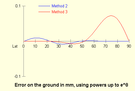
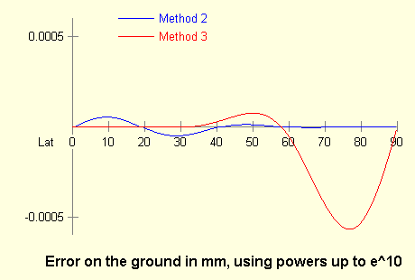
For a method that suits all latitudes, it seems best therefore to use either iteration or Method 2. The maximum error on the ground with Method 2 is as follows:

Highest power of e included	6	8	10	12
Maximum error on ground in mm	1.9	0.010	5.9 × 10−5	3.4 × 10−7

Reference

[1] http://mathworld.wolfram.com/IsometricLatitude.html