The “spherical blackboard” is an elementary part of the statistical theory of shape developed by the late David Kendall and his collaborators. It helps to answer questions of the kind: if a triangle is formed by three points placed at random in a plane region, what is the probability that the triangle belongs to a certain class of shapes?

These notes attempt to explain the theory of the spherical blackboard from an elementary point of view. The theory is then applied to answer the question: If three sites have independent uniform distributions inside a circle or square, what is the probability that the triangle is nearly right-angled, i.e. contains an angle in the range [π/2−ε,π/2+ε], where ε is a predefined small tolerance? This question arises e.g. from F. W. Holiday’s book The Dragon and the Disc, which draws attention to large right-angled triangles formed by ancient sites in the landscape. (Such theories of leys and landscape geometry are discussed statistically in Bob Forrest’s essay The Linear Dream.)

Definition of a shape

The full theory of shape [Ref. 1] applies to any number of points in any number of dimensions. These notes are confined to 2 dimensions and for the most part to 3 points.

An ordered set of n points in the plane (n≥2) has a shape, in Kendall’s sense, provided only that the n points do not all coincide. Let (P₁,…,P_n) and (Q₁,…,Q_n) be two such ordered sets; these sets of points have the same shape iff there is a combination of rotation, translation and scaling (dilatation) that takes P_j to Q_j ( j=1,…,n). Formally: if we express this relation by (P₁,…,P_n)∼(Q₁,…,Q_n), then ∼ is clearly an equivalence relation, and the shape of (P₁,…,P_n) is the equivalence class to which it belongs.

Note that the labelling (i.e. ordering) of the points is important. In Fig. 1, the two sets of points (A,B,C) form congruent triangles but have different shapes, in Kendall’s sense, because the labelling is different.

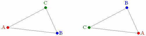
The 6 ways of labelling a given triangle will usually produce 6 different shapes. The exceptions are: equilateral triangle (2 shapes); and collinear triangle with one point midway between the other two (3 shapes).

The distance between two n-point shapes

Let (x_j,y_j) and (u_j,v_j) ( j=1,2,…,n) represent two n-point shapes. Keeping the (u_j,v_j) fixed, we transform the (x_j,y_j) into (x_j′,y_j′) by translation, scaling and rotation so as to minimize

∑[(xj′−uj)2+(yj′−vj)2].

By definition of shape, the minimum value will be 0 iff the sets (x_j,y_j) and (u_j,v_j) have the same shape. In general, the minimum value, with suitable scaling, can be used to define a distance between the shapes.

Consider first translation alone. The optimal translation (a,b) is that which minimizes

∑[(xj+a−uj)2+(yj+b−vj)2]

=na2+2a∑(xj−uj)+nb2+∑(yj−vj)+ const,

and this is minimized by a=∑(x_j−u_j)/n,  b=∑(y_j−v_j)/n. Hence a necessary condition for a minimum is that the centroid of the (x_j,y_j) should coincide with the centroid of the (u_j,v_j). From now on, assume that this condition holds, and assume w.l.o.g. that the common centroid is at the origin.

Rotation and scaling can be dealt with together, by considering the transformation

(xj,yj)→(αxj−βyj,βxj+αyj),

where α and β are chosen to minimize

∑[(αxj−βyj−uj)2+(βxj+αyj−vj)2]

=(α2+β2)∑(xj2+yj2)−2α(∑(xjuj+yjvj)−2β(∑(xjvj−yjuj)+∑(uj2+vj2).

Since ∑(x_j²+y_j²)≠0 (else the (x_j,y_j) would all coincide, contrary to hypothesis) the minimum is attained by taking

α= ∑(xjuj+yjvj) ,  β= ∑(xjvj−yjuj) ∑(xj2+yj2) ∑(xj2+yj2)

and the minimum value is

∑(uj2+vj2) −  [∑(xjuj+yjvj)]2  −  [∑(xjvj−yjuj)]2 . ∑(xj2+yj2) ∑(xj2+yj2)

This value depends on the scaling of the (u_j,v_j), but if we divide by ∑(u_j²+v_j²) we can define the squared distance between the shapes by

D2=1 −  [∑(xjuj+yjvj)]2+[∑(xjvj−yjuj)]2 , ∑(xj2+yj2)∑(uj2+vj2)

(1)

where 0≤D≤1. This definition assumes that the centroids of the point sets (x_j,y_j) and (u_j,v_j) are at the origin, but is independent of scaling and rotation.

If we identify the points with complex numbers, say z_j=x_j+iy_j, w_j=u_j+iv_j,  then

D2=1 −  |∑zjwj*|2 ∑|zj|2 ∑|wj|2

where * denotes the complex conjugate.

We have not shown that the distance D so defined satisfies the triangle inequality, but for n=3 this will follow from the discussion below, in which D is identified with a certain distance in 3-dimensional Euclidean space.

The distance between two triangular shapes

The following way of defining a triangle shape is often used in the literature. Fix a distance k>0, which is to be the same for all triangles. Given a triangle ABC, scale so that AB=2k. (Here we must exclude the triangle shape that has A=B, but this is not a serious restriction.) Take the origin of (x,y)-axes at the centroid G, with Gx parallel to AB (see Fig. 2).

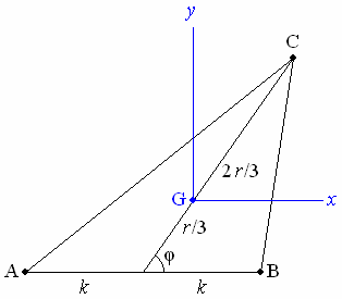
Let the median through C have length r, so that GC=2r/3, and let φ be the direction of GC, measured anticlockwise from the x-axis.

Clearly the shape of the triangle is determined by r and φ. Given two such shapes, determined by (r₁,φ₁) and (r₂,φ₂) respectively, a short calculation shows that the ditance D between the shapes is given by

D2=  3k2 [r12+r22−2r1r2cos(φ1−φ2)]. (3k2+r12)(3k2+r22)

This suggests the choice k=1/√3. The distance can then be put as

D2=  1 [ 1−  1−r12   1−r22  −  2r1   2r2 cos(φ1−φ2) ] . 2 1+r12 1+r22 1+r12 1+r22

If for j=1,2 we set r_j=tan(θ_j/2), where 0≤θ_j<π, then the last equation becomes

D2=  1 [1−cosθ1 cosθ2−sinθ1 sinθ2 cos(φ1−φ2)]. 2

It is easy to check that this is the distance between two points (φ₁,θ₁) and (φ₂,θ₂) on a sphere of radius 1/2, where φ is the longitude and θ is the co-latitude (i.e. π/2− latitude). This observation by Kendall is the basis of the “spherical blackboard”.

The distance D so defined is the distance along the chord between the two points. Kendall [Ref. 2] uses the distance along the surface of the sphere, which is sin⁻¹D.

Representing triangle shapes on a sphere

We have seen that the triangle shape defined by (r,φ), as in Fig. 2, corresponds to the point (θ,φ) on a sphere of radius 1/2, where r=tan(θ/2). This correspondence can be defined in a simple geometrical way, as in Fig. 3.

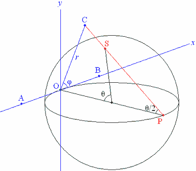
Here O is the pole θ=0 on the sphere and P is the opposite pole θ=π. In the tangent plane at O take (x,y)-axes so that Ox lies in the plane φ=0 and Oy lies in the plane φ=π/2. Since OP=1, the point C=(r,φ) in the plane corresponds to S=(θ,φ) on the sphere by stereographic projection from P. The point P itself does not correspond to any point in the plane; it corresponds however to the missing triangle shape with A=B.

In the literature, a probability density on the sphere may be expressed in terms of a probability density in the (x,y) plane. To convert between them, note that a small element of area δA at S is projected into an element of area (1+r²)²δA at C, where r=OC.

The probability of a near-right-angled triangle

First consider the locus on the sphere of triangle shapes ABC in which angle C has a given value χ and the points A,B,C run (say) anticlockwise. In the (x,y) plane (Fig. 3), the locus of C is clearly a circular arc with endpoints at A and B. Since stereographic projection preserves circles, the locus on the sphere is a circular arc with endpoints at the projections A′ and B′ of A and B.

In Fig. 4, Ω is the centre of the sphere and N is the pole of the circular arc C=χ. Points on the arc are parametrized by the longitude ω measured w.r.t. N, from the centre of the arc. It is straightforward to show that the ends of the arc are ω=±ω₀ , where

ω0=cos−1 ( −  1 cosχ ) . 2

For small ε, shapes with χ<C<χ+ε lie in the narrow lune shown in Fig. 4. The width of the lune at the point with parameter ω is found to be ε√3(2cosω+cosχ)/2(3+sin²χ), and the radius of the arc C=χ is √3/2(3+sin²χ)^1/2. Hence, for a given probability density on the sphere, the probability that χ<C<χ+ε, with A,B,C running anticlockwise, is

ε× ∫ ω0 3(2cosω+cosχ) ƒ(ω)dω, −ω0 4(3+sin2χ)3/2

(2)

where ƒ(ω) is the probability density at the point with parameter ω.

Right-angled triangles

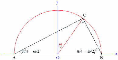
The case of a right angle at C (i.e. χ=π/2) is simpler than the general case. The arc C=π/2 is a semicircle in a plane parallel to the (x,y) plane of the stereographic projection. In the (x,y) plane, therefore, the angle ω is preserved (see Fig. 5), and the other angles of the triangle are given by A=π/4−ω/2, B=π/4+ω/2.

The method above will now be applied for χ=π/2 and two particular shape densities on the sphere, namely those generated when A,B,C have independent uniform distributions in a circular region and a square region respectively. First, the probability that π/2<C<π/2+ε, with A,B,C running anticlockwise, is obtained by putting χ=π/2 in formula (2). This gives ω₀=π/2 and simplifies the fraction in (2) to 3cosω/16.

We then need to

• Multiply by 2 for the probability that |C−π/2|<ε;
• Multiply by 2, since A,B,C running clockwise is equally acceptable;
• Multiply by 3, since any of the angles A,B,C close to ±π/2 is acceptable. (We ignore the small probability that triangle ABC has two angles very close to a right angle.)

The probability that triangle A,B,C has an angle within ε of a right angle is thus

ε×  9  ∫ π/2 cosω ƒ(ω)dω. 4 −π/2

(3)

Circular region

The shape density m_circle when A,B,C have independent uniform distributions in a circle was found by Kendall [Ref. 2] (or see alternative proof on this website). His shape density m is scaled so that its integral over the sphere equals the surface area of the sphere, i.e. π. For the probability density we therefore need to divide Kendall’s m by π. Define a function K by

K(α) =  1 ∫ α sin4 ψ dψ =  1 ( 3 α−  1 sin 2α+  1 sin 4α ) . sin4α 0 sin4α 8 4 32

At the triangle whose angles are A,B,C the probability density on the sphere is then

8  [sin2A+sin2B+sin2C]2 [K(A)+K(B)+K(C)]. 9π2

This is in effect Kendall’s formula (20) except for π² in the denominator instead of π.

In our case, sin²A+sin²B+sin²C=2, so the probability density at the point parametrized by ω is

ƒ(ω) =  32 [ K ( π  −  ω )  + K ( π  +  ω )  + K ( π ) ] . 9π2 4 2 4 2 2

Since K(π/2)=3/16 and ƒ(ω) is here an even function of ω, the probability of an angle within ε of a right angle is obtained from (3) as

ε×16 ∫ π/2 cosω [ K ( π  −  ω )  + K ( π  +  ω )  +  3π ] dω. 0 4 2 4 2 16

Noting that

sin2(π/4±ω/2)=[1−cos(π/2±ω)]/2=(1±sinω)/2=(1∓sinω)/2cos2ω,

we find after a short calculation that the integrand equals

1−3ωsec2ωtanω−3sec2ω+  3π (secωtan2ω+sec3ω)+  3π cosω, 4 16

of which the indefinite integral is

I(ω)=ω−  3 ωsec2ω−  3 tanω+  3π secωtanω+  3π sinω. 2 2 4 16

Here I(ω) appears to have a singularity at ω=π/2, but one easily checks that, for small δ, I(π/2−δ)=5π/16+O(δ). Since I(0)=0, the definite integral is 5π/16, and so the probability of a near-right angle is 5ε/π.

Conclusion: If points A,B,C have independent uniform distributions in a circular region, and ε is a small angle, then the probability that triangle ABC has an angle within ε of a right angle is (5/π)ε. This conclusion has been confirmed by computer simulations.

Square region

The shape density for three points A,B,C with independent uniform distributions in a square was found by Kendall & Le [Ref. 3], who express it in terms of the (x,y)-coordinates in the plane of the stereographic projection. Here the density is scaled so that its integral over the plane is 1, so there is no need to divide by π as was done for a circular region. The formula for the shape density is complicated, and takes different forms in different regions of the plane. These regions are of four kinds, which Kendall & Le label A, B, C, D as in Fig. 6. The shape densitiy and its first two derivatives are continuous between regions; higher derivatives are not necessarily so.

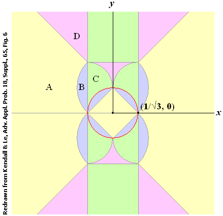
This looks daunting, but the locus of points C such that triangle ABC has a right angle at C turns out to be the circular boundary between regions of Type B and C (red in Fig. 6). Hence the shape density for either Type B or Type C can be used throughout. We here use the density for Type B, which is the simpler of the two.

Kendall & Le set

a=x√3, b=y√3, u=1+a, v=1−a.

In a region of Type B with a≥0,  b≥0,  a+b≥1,  a²+b²≤1 (i.e. for 0≤ω≤π/2 in our notation), their expression for the shape density is

v3b−2u−3/30  + v5b−4u−1/40  − v2b−1u−3/5  + v3b−2u−2/20  − v4b−3u−1/20  + u−3  − 2bu−3/3  + b2u−3/4  − b3u−3/20  − v2b−1u−2/5  + v3b−2u−1/20  − 3v2b−1u−1/20  + u−1/4  − 3bu−1/20.

For our application we need to feed in x=(1/√3)sinω, y=(1/√3)cosω. Also, as noted in the section on stereographic projection, to get the probability density on the sphere we need to multiply by (1+r²)², with r=1/√3 in our case. The probability density on the sphere works out to

ƒ(ω)=  2  [199+220sinω+46sin2ω+12sin3ω+3sin4ω−16cosω(11+8sinω)]. 135(1+sinω)4

This is valid for ω in [0,π/2], which is enough since ƒ(ω) is clearly an even function of ω. We next need to integrate cosωƒ(ω). For the terms in ƒ(ω) with a factor cosω put t=tan(ω/2−π/4) to get

∫ cos2ωdω  =  1 t3+  1 t5,  ∫ cos2ωsinωdω  =  1 t3−  1 t5. (1+sinω)4 6 10 (1+sinω)4 6 10

The rest of the integration is straightforward if we rewrite the polynomial in sinω as a polynomial in (1+sinω) (there is then no cubic term, and hence no logarithm in the integral). The probability of a near-right angle is obtained from (3) as

ε×  9 ∫ π/2 cosω ƒ(ω)dω =  116ε . 2 0 75

Conclusion: If points A,B,C have independent uniform distributions in a square region, and ε is a small angle, then the probability that triangle ABC has an angle within ε of a right angle is (116 / 75)ε. This conclusion has been confirmed by computer simulations.

The probability of a near-right angle in a square region (about 1.546667ε) is somewhat less than in a circular region (about 1.591549ε)

[1]	D. G. Kendall, D. Barden, T. K. Carne & H. Le, Shape and Shape Theory, Wiley, 1999.
[2]	D. G. Kendall, “Exact distributions for shapes of random triangles in convex sets”, Advances in Applied Probability, 17, 308–329 (1985).
[3]	David G. Kendall & Hui-Lin Le, “Exact shape-densities for random triangles in convex polygons”, Advances in Applied Probability, 18, Supplement, 59–72 (1986).