The typescript of these notes is dated 18 June 1977.
As the last sentence shows, this was in the days before computers became available to all.
A proof is given of the “strip formula” for estimating the number of chance alignments
in a random set of sites. The sites are supposed to be discs, all the same size, and a set of sites is
considered to be aligned if a straight line can be drawn that intersects all the discs.
Equivalently, we can consider the sites to be geometrical points, and a set of points is aligned if
they can be covered by a movable strip of the same width as the discs.
In the 1985 notes
the formula is generalized to allow discs of different sizes
(in which case the term “strip formula” is no longer appropriate).
MB, May 2013
This problem arises from the work of Alfred Watkins,
who asserted that ancient sites such as churches, beacons, mounds, markstones, etc.
could be shown on the map to fall into straight alignments. Watkins believed that
these lines, which he called “leys”, marked the course of ancient trackways that
were constructed in prehistoric times and were still discernible in places.
He tried to show by experiment that the alignments were more numerous than chance
would allow, but his method is questionable (see below).
The problem. Let n points P1,P2,…,Pn be placed
independently and at random (uniform p.d.f. with respect to area) inside a bounded convex
plane region R. A “critical distance” c is decided on, and then a set of points such as
P1,P2,…,Pr is said to form an r-point alignment if and only if
there exists a straight line passing within distance c of each Pi. It is assumed
that c is small compared with the dimensions of R. Given R, c, n, and r,
what is the expected number of r-point alignments?
Three equivalent statements of the alignment criterion are:
- (a) About each Pi as centre draw a circle of radius C; then P1, …, Pr
are aligned iff a straight line can be drawn so as to cut all the circles.
- (b) P1, …, Pr are aligned iff a movable infinite strip of width 2c
can be placed so as to cover all the Pi.
- (c) P1, …, Pr are aligned iff the minimum width of their convex hull
is less than 2c.
Although (b) is used below, note that (a) gives a method for dealing with sites of non-zero dimensions,
e.g. churches. Each site can be replaced by a circle of radius c that wholly contains it.
An objective method of fixing the exact position of the circle is to make it concentric with
the smallest circle that wholly contains the site.
If e.g. P1P2P3P4P5 is a 5-point alignment there will be five 4-point subalignments
such as P1P2P3P4 and ten subalignments such as P1P2P3. A maximal alignment is
one that is not part of some alignment of higher order. Given R and c, let e(n,r)
be the expected number of r-point alignments among n points, and let e′(n,r)
be the expected number of maximal r-point alignments. In these notes, only e(n,r)
is calculated. I do not know how to find e′(n,r), though it is easy to see that
| e(n,r)−(r+1)e(n,r+1)<e′(n,r)<e(n,r). |
|
Calculation of e(n,r). Recall (i) that R is convex, (ii) that c is small
compared with the dimensions of R (e.g. in practice R might be 40 km square
with c = 20 m). Given R and c, let n points P1, …, Pn be placed
randomly inside R. Let p(r) be the probability that P1, …, Pr form an alignment
with endpoints Pr−1 and Pr. Then
| e(n,r)= |
( |
n |
) |
( |
r |
) |
p(r). |
| r |
2 |
|
(1) |
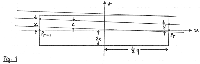
Denote the distance Pr−1Pr by q and let ƒ(q) be the p.d.f. of q. A necessary
condition for P1,…,Pr to form an alignment with endpoints Pr−1 and Pr
is that P1,…,Pr−2 fall inside the q×4c rectangle shown in Fig. 1.
In view of assumptions (i) and (ii) we may assume
(iii) that q≫c
(iv) that the rectangle in Fig. 1 lies wholly inside r.
That is, we ignore the small proportion of cases in which (iii) or (iv) is false.
Let A be the area of R; then the probability that P1,…,Pr−2 all fall inside the rectangle is
| ∫ |
∞ |
(4cq/A)r−2ƒ(q)dq=(4c/A)r−2Mr−2 |
| 0 |
|
where Mr−2 is the (r−2)nd moment of f. Now assume that P1,…,Pr−2 are placed
independently and at random inside the rectangle, and let the centre line of a movable strip
meet the ends of the rectangle at (−½q,x) and (½q,y). Since q≫c, Pr−1 and Pr
will lie inside the strip iff
If a typical Pi (1≤i≤r−2) has coordinates (ui,vi) then Pi will lie
inside the strip iff
| |vi−((½q−ui)x+(½q+ui)y)/q|<c. |
|
(3) |
Setting
and
we can rewrite (3) as
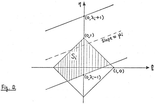
Each position of the strip corresponds to some point in the (ξ,η) plane according to (4).
Inequalities (2) hold iff (ξ,η) lies inside the infinite strip whose boundaries have slope
μi and cut the η-axis at (0,λ±1). Hence the movable strip in the (u,v) plane
covers Pr−1, Pr and Pi iff the corresponding (ξ,η) lies inside the shaded region Si.
The points P1,…,Pr form an alignment iff
We find the probability that (7) holds. Since the (ui,vi) have independent uniform p.d.f.s
inside the rectangle, (5) implies that the λi and μi have independent uniform p.d.f.s in
|λi|<2, |μi|<1. Hence the procedure for getting Si can be restated as follows:
The boundary line cutting the square has the equation
where μi, νi have independent uniform p.d.f.s in (−1,1); and then Si can lie either
above or below the boundary line, each with probability 1½.
Lemma 1.Given i and j (1≤i<j≤r−2)
the probability that the boundary lines
of Si and Sj meet inside the square is 1/3.
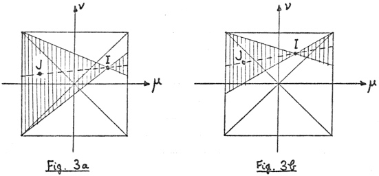
Proof.Let these lines meet at (ξ0,η0). This point lies inside the square
iff |η0−ξ0|<1 and |η0+ξ0|<1. In the (μ,ν)-plane the points
I=(μi,νi) and J=(μj,νj) have independent uniform p.d.f.s in the square
|μ|<1, |ν|<1. It is easy to verify that IJ produced meets the left and right sides
of the square at (−1,η0−ξ0) and (+1,η0+ξ0). Hence we want the probability that IJ
produced meets both sides internally. By symmetry we may assume that I lies in one of the regions
| 0<|νi|<μi<1 (Fig. 3a) |
| 0<|μi|<νi<1 (Fig. 3b) |
|
Then J is required to lie in the shaded region, and the probability that this occurs is
| 1 |
∫ |
1 |
∫ |
μ |
(1+μ2)dμdν |
+ |
1 |
∫ |
1 |
∫ |
ν |
(1−ν)(1+μ2)dμdν |
| 2 |
μ=0 |
ν=−μ |
2(1+μ) |
2 |
ν=0 |
μ=−ν |
2(1−μ2) |
|
| = |
( |
11 |
− |
ln 2 |
) |
+ |
( |
ln 2 |
− |
7 |
) |
= |
1 |
. |
| 12 |
12 |
3 |
|
Lemma 2. Let C be a plane convex region.
Given a set of s straight lines, all cutting C,
let t be the number of intersection points inside C (no multiple intersections). Then the s
lines divide C into s+t+1 non-empty regions.
Proof. For s=1 or 2 the result is clear.
Suppose the result holds for a given set of s lines.
Add a new line L, and let L meet Δt of the s lines inside C. Then C∩L is divided into
Δt+1 segments, each of which divides one of the s+t+1 regions of C into two parts.
Hence the number of regions is now
| (s+t+1)+(Δt+1)=(s+1)+(t+Δt)+1. |
|
The result follows by induction.
Now take C to be the square of Fig. 2, and fix a set of r−2 boundary lines for the Si.
Let t intersection of the lines be inside C, with no multiple intersections. Then by Lemma 2
C is divided into r−1+t non-empty regions. Since each Si can be either above or below
its boundary line, the set of Si can be defined in 2r−2 ways. These are all equally
probable, so that
If the μi and νi are now allowed to vary, Lemma 1 implies that E(t)=(r−2)(r−3)/6.
Multiple intersections have zero probability and can be ignored. Hence
| pr( | ∩ | Si≠∅)=(r−1+E(t))/2r−2=r(r+1)/(3⋅2r−1). |
|
Combining the above results we find that
Values of Mr−2 in two particular cases
(1) Circle of radius a:
| Mr−2= |
2Γ(r)ar−2 |
| Γ(½r+1)Γ(½r+2) |
|
(2) Rectangle of sides a and b:
Let d=√(a2+b2), α=a/d, β=b/d,
| H1= |
1 |
ln |
( |
1+β |
) |
, |
K1= |
1 |
ln |
( |
1+α |
) |
, |
| β |
α |
α |
β |
|
|
|
| Hr= |
1+(r−2)α2Hr−2 |
, |
Kr= |
1+(r−2)β2Kr−2 |
(r=3,4,…). |
| (r−1) |
(r−1) |
|
Then
| Mr−2= |
4dr−2 |
( |
Hr+Kr− |
1−αr+2−βr+2 |
) |
. |
| r(r+1) |
(r+2)α2β2 |
|
Practical calculation
In practice it is convenient to denote the area of R by k2.
The expected number of r-point alignments among n points, with each of the r points allowed
to be off-line by a distance not exceeding c, is given by
| e(n,r)=n(n−1) … (n−r+1)⋅(c/k)r−2⋅G(r) |
|
where the factor G(r) depends only on r and the shape of the region R.
For any particular shape G(r) can be tabulated once for all, thus:
| |
Circle | Square* | 9:8 rect.† | 3:2 rect. | 2:1 rect. |
|---|
| G(3) |
1.0217 | 1.0428 | 1.0456 | 1.0754 | 1.1381 |
| G(4) |
1.0610 | 1.1111 | 1.1188 | 1.2037 | 1.3889 |
| G(5) |
0.7433 | 0.8024 | 0.8126 | 0.9269 | 1.1888 |
| G(6) |
0.3940 | 0.4407 | 0.4494 | 0.5488 | 0.7907 |
| G(7) |
0.1683 | 0.1962 | 0.2016 | 0.2651 | 0.4312 |
| G(8) |
0.06020 | 0.07365 | 0.07630 | 0.1084 | 0.1992 |
| G(9) |
0.01855 | 0.02398 | 0.02505 | 0.03851 | 0.07982 |
| G(10) |
0.005019 | 0.006910 | 0.007280 | 0.01209 | 0.02822 |
| G(11) |
0.001211 | 0.001790 | 0.001901 | 0.003402 | 0.008921 |
| G(12) |
0.0002637 | 0.0004217 | 0.0004513 | 0.0008680 | 0.002551 |
*O.S. 1:50 000 maps cover 40×40 km.
†O.S. 1-inch (1:63 360) maps cover 45×40 km.
Example. On 1:50000 Sheet 154 there are 165 old churches, excluding those in Cambridge city.
If the critical distance c is 20 m, find the expected number of 5-point alignments.
According to the formula, the expected number is
| 165×164×163×162×161×(20/40000)3×0.8024=11.5 |
|
Watkins’s experiments. To find to what extent alignments of sites might occur by chance,
Watkins carried out a few rough practical tests.
One of these is described in The Old Straight Track as follows:
“This is in the Andover map (Sheet 283) which contains 51 churches, and there are on it no less than
8 separate instances of 4 churches falling in a straight line, in addition to the example of 5 churches
in alignment already mentioned. To test the argument that this might be accidental I took a similar sized
sheet of paper and marked 51 crosses in haphazard distribution over it. Only one instance could be found on this of
4 points aligning, and none of 5.”
The map Watkins was using measures 18×12 inches, but he doesn’t say how accurate an alignment had to be
before he included it. If we take his result at face value, we can get a rough idea by working out what
value of c would make the number of 4-point alignments equal to 1. This turns out to be surprisingly small,
namely c=0.0055 in. = 0.14 mm.
In Archaic Tracks Round Cambridge Watkins describes a similar experiment and states that
“only one or two”
4-point alignments were found on “a large sheet with a hundred points”.
This is vague, but we can get an idea
of the tolerance allowed, by assuming a sheet 18×12 inches as before and the expected number of 4-pointers
equal to 1.5. Then c=0.0017 in. = 0.043 mm, a distance scarcely perceptible
to the naked eye.
But Watkins also says here that on average a 3-pointer comes when only nine marks are made on a sheet.
This implies c=0.027 in = 0.69 mm, which is not only much larger than before
but also seems more likely to indicate Watkins’s true standard of accuracy. Why then the discrepancy?
The suspicion must be that with 50 or 100 crosses on his sheet Watkins thought he had counted all the chance
4-pointers when in fact many more remained to be discovered. To find all the alignments among a large number of points
is a very long job. (I once decided to find all 3-point alignments of mounds on the 1:50 000 Cambridge map.
Chance alone would yield about 60, but it took so long to find even 5 or 6 that I abandoned the task.
A computer is really needed.)