Random triangles in a bounded measurable set

These notes were written nearly 30 years ago. They were not meant for publication, but are put on this website because David Kendall mentions them in [Ref. 2]. They provide an alternative derivation of Kendall’s formula for the shape density of a random triangle formed by 3 points with independent uniform distributions inside a circle. MB, May 2013

Let K be a bounded measurable set in R² with |K|>0. Let three distinguishable points A,B,C have independent uniform distributions in K. We describe a method for finding the shape distribution of triangle ABC, where following Kendall [Ref. 1] the shape is identified with a point σ on S²(½) (surface of the 3-dimensional sphere of radius ½). We use spherical coordinates θ (co-latitude) and φ (longitude) on S²(½) identical with those on page 97 of [Ref. 1]. The total measure of S²(½) is taken to be 1, so that

dσ =  1  sinθ dθ dφ . 4π

(1)

Suppose first that A,B,C have independent identical circular gaussian distributions in R², say

prob(x,y)=λ exp(−λπ(x2+y2)) dx dy,

(2)

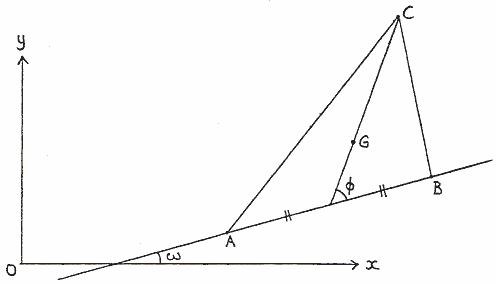
where the origin 0 has any convenient location w.r.t. K. Since K is bounded, the induced distribution over K will tend uniformly to the uniform distribution as λ→0. The required shape distribution over K can therefore be obtained as the limit of the shape distribution induced by (2). The positions of A,B,C are determined by the six coordinates x_A,y_A, etc, or alternatively by the following:

(a) the shape σ of triangle ABC;
(b) the coordinates (x_G,y_G) of the centroid G;
(c) the size g defined by

g=√(|GA|2+|GB|2+|GC|2) ;

(3)

(d) the orientation ω measured w.r.t. any convenient origin.

We use the notation of Fig. 1. As shown in [Ref. 1], or on this website, the position of the shape ABC on S²(½) (the “spherical blackboard”) is given by

• longitude = φ (with φ<0 if A,B,C run clockwise);
• co-latitude = θ, where

|GC|:|AB|=sin(θ/2):√3cos(θ/2) .

(4)

We next find the joint p.d.f. of σ,G,g,ω. It follows from (3) and (4) that

xA=xG−  1 g sin(θ/2) cos(φ+ω)  −  1 g cos(θ/2) cosω √6 √2 yA=yG−  1 g sin(θ/2) sin(φ+ω)  −  1 g cos(θ/2) sinω √6 √2 xB=xG−  1 g sin(θ/2) cos(φ+ω)  +  1 g cos(θ/2) cosω √6 √2 yB=yG−  1 g sin(θ/2) sin(φ+ω)  +  1 g cos(θ/2) sinω √6 √2 xC=xG−  2 g sin(θ/2) cos(φ+ω) √6 yC=yG−  2 g sin(θ/2) sin(φ+ω) √6

(5)

and from (3) that

(xA2+yA2)+(xB2+yB2)+(xC2+yC2)=3xG2+3yG2+g2 .

(6)

The Jacobian of (5) turns out to have absolute value

| ∂(xA,yA,xB,yB,xC,yC) |  =  3 g3 sinθ , ∂(xG,yG,g,θ,φ,ω) 4

(7)

so from (1) and (6) the required p.d.f. is

prob(σ,G,g,ω)=3πλ3g3 exp(−πλ(3xG2+3yG2+g2)) dσ dG dg dω.

(8)

Here the function on the RHS is independent of ω and σ. This shows that the orientation ω is uniformly distributed, as expected, and also that the circular gaussian induces a uniform distribution of the shape σ on S²(½), as already shown by Kendall in [Ref. 1].

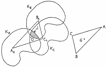
Now consider some fixed shape, size and orientation σ,g,ω of ABC. Conditionally on these, the centroid G ranges over R² with the circular gaussian distribution implied by (8). We need the probability that all three points A,B,C then fall inside K. Define points A₀,B₀,C₀ such that OA₀ = AG, etc. Then A₀B₀C₀ is a fixed triangle congruent to ABC and rotated through π w.r.t. ABC (Fig. 2).

Let K_A,K_B,K_C be the sets obtained by translating K through the vectors OA₀, OB₀, OC₀, and define

J=J (σ,g,ω)=KA∩KB∩KC .

(9)

Then clearly A,B,C, all fall in K if and only if G falls in J. Since K is measurable, so is J. Now keep σ fixed and allow g and ω to vary. Then from (8) the probability that A,B,C all fall in K is

dσ ∫ ∞ ∫ 2π 3πλ3g3exp(−πλg2)(1+O(λ)) |J (σ,g,ω)| dg dω. g=0  ω=0

(10)

Since K is bounded there is some g₀>0, independent of σ and ω, such that |J (σ,g,ω)|=0 whenever g>g₀ (because ABC is then too large to fit inside K in any position). Hence the exponential in (10) can be absorbed into the term 1+O(λ), and that term can then be taken outside the integral since O(λ)→0 uniformly over all ω and g≤g₀. The overall probability that A,B,C all fall in K is

λ3 |K|3 (1+O(λ)).

(11)

Dividing (10) by (11) and letting λ→0 we get the desired p.d.f.

prob(σ)=3π|K|−3dσ ∫ ∞ ∫ 2π g3 |J (σ,g,ω)| dg dω. g=0  ω=0

(12)

Recall that in Fig. 2 the size of A₀B₀C₀ is the variable g while K_A,K_B,K_C are congruent to K. It may be more convenient to apply the dilatation ƒ=g⁻¹ to Fig. 2 so that A₀B₀C₀ has size 1 while K_A,K_B,K_C undergo equal dilatations ƒ about A₀,B₀,C₀. Define

I (σ,ƒ,ω)=ƒKA∩ƒKB∩ƒKC .

(13)

Then

|J (σ,g,ω)|=ƒ−2|I (σ,ƒ,ω)|

(14)

and (12) can be rewritten as

prob(σ)=3π|K|−3dσ ∫ ∞ ∫ 2π ƒ−7 |I (σ,ƒ,ω)| dƒ dω, ƒ=0  ω=0

(15)

where the integrand vanishes for all ƒ<g₀⁻¹.

If K is star-shaped a further transformation is possible. Take O to be one of the points from which the whole boundary of K is visible. For any P∈R² define

ƒ*=ƒ*(P,ω)=inf{ƒ|P∈I (σ,ƒ,ω)} .

(16)

Then P∈I (σ,ƒ,ω) for all ƒ>ƒ_* and the contribution to (15) for a given P and ω is

dP dω  ∫ ∞ ƒ−7dƒ=  1 ƒ*−6dP dω. ƒ* 6

(17)

Hence (15) can be rewritten for star-shaped K as

prob(σ)=  π |K|−3dσ ∫   ∫ 2π ƒ*(P,ω)−6 dP dω . 2 P∈R2 ω=0

(18)

If one were interested in some statistic other than shape, e.g. the minimum width of triangle ABC as a criterion for approximate alinement, one could perhaps apply a similar method with integration over a suitable combination of σ,g,ω. This has not yet been tried.

Applications

Since triangle A₀B₀C₀ has the same shape as ABC we can and will drop the suffix 0 from now on. As an external check on the method we calculate the shape distribution when K is a circular disk; this has already been done by Kendall [Ref. 2]. Let K have radius 1 and centre at O. The intersection J, when non-empty, is bounded by three circular arcs, and the expression for | J | is complicated. It is easier to use formula (18), where now f_*(P,ω) is independent of ω and equals the distance from P to the furthest vertex of ABC.

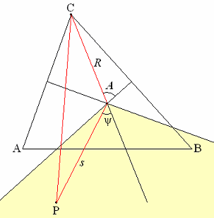
Suppose first that A,B,C are not collinear. The set of P for which C (say) is the furthest vertex forms an infinite wedge W  (Fig. 3, shaded) bounded by the perpendicular bisectors of CA and CB. The function f_*(P,ω) in (18) is now |CP|. Fig. 3 shows that

∫   |CP|−6 dP  =  ∫ A ∫ ∞ s ds dψ  . W ψ=−B s=0  (s2+2Rscosψ+R2)3

(19)

We find first that

∫ ∞ s ds  =  1 (3−3ψcotψ−sin2ψ) s=0  (s2+2Rscosψ+R2)3 8R4sin4ψ

(20)

(where the RHS is O(1) for small ψ). Hence

∫   |CP|−6 dP  =  1 [t(A)csc4(A)+t(B)csc4(B)] , W 4R4

(21)

where R is the circumradius of ABC, given by

4R2(sin2A+sin2B+sin2C)=3 ,

(22)

and the function t is given by

t(A)=  3 A−  1 sin2A+  1 sin4A . 8 4 32

(23)

Integration over ω contributes a factor 2π, so that (18) yields, after summing over A,B,C,

prob(σ)=  8 (∑sin2A)2 ∑t(A)csc4A dσ . 9π

(24)

This formula is the same as that given by equations (20) and (21) of [Ref. 2]. It is interesting to note that the function we have called t(A) is obtained by Kendall in a different way, namely as

t(A)=  ∫ A sin4ψ dψ . 0

(25)

When ABC degenerates into a straight line, say with C between A and B, then the contribution from C vanishes and (18) becomes the sum of two equal integrals over half-planes separated by the perpendicular bisector of AB. If following [Ref. 2] we write

|AC|:|CB|=q:p, p+q=1 ,

(26)

then we easily find

prob(σ) =  1 (1+p2+q2)2 dσ , 3

(27)

again in agreement with [Ref. 2].

[1]	D. G. Kendall, “Shape manifolds, procrustean metrics, and complex projective spaces”, Bull. London Math. Soc. 16, 81–121 (1984).
[2]	D.G. Kendall, “Exact distributions for shapes of random triangles in convex sets”, Adv. Appl. Prob. 17, 308–329 (1985).