This webpage is typed up from undated notes (probably 1980s).
Although I haven’t yet found a reference to the main result
in the literature, it is unlikely to be original.
MB, January 2014
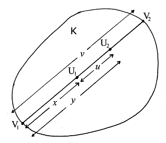
Let K be a bounded plane convex region (fig. 1).
Let points U1 and U2 have independent uniform distributions inside K.
Let U1U2 produced meet the boundary of K at V1 and V2,
where (to avoid ambiguity) V1→V2 has azimuth in the range [0,π).
Let U1U2=u with PDF ƒ(u);
let V1V2=v with PDF g(v);
let V1U1=x and V1U2=y.
1. Given v and x, to find the PDF of y
i.e. to find the probability that y<V1U1<y+δy, where δy is small.
The probability that V1V2=v and V1U1=x exactly is 0; so assume
v<V1V2<v+δv and x<V1U1<x+δx,
where δv and δx are small compared with δy.
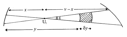
Given U1, the permissible set of azimuths of U1U2 will be a (possibly empty) union
of small intervals like ε in fig. 2.
(The diagram is drawn for x<y; the change for x>y is straightforward.)
The shaded area shows the posssible positions of U2. Hence
| prob(y1<V1U2<y+δy)= |
|y−x|⋅ε⋅δy |
= |
|y−x|δy |
. |
| ½εx2+½ε(v−x)2 |
x2−vx+½v2 |
|
Thus for 0≤y≤v the PDF of y for a given v and x is
2. Given v, to find the PDFs of x and y
Clearly x and y have identical PDFs for a given v; call this PDF φv.
From section 1 we get
| φv(y)= |
∫ |
v |
|y−x|φv(x)dx |
. |
| x=0 |
x2−vx+½v2 |
|
Put φv(x)=ψ(x)(x2−vx+½v2) and rewrite the last equation as
| (y2−vy+½v2)ψ(y)= |
∫ |
y |
(y−x)ψ(x)dx− |
∫ |
v |
(y−x)ψ(x)dx. |
| x=0 |
x=y |
|
Differentiate twice with respect to y:
| (y2−vy+½v2)ψ′(y)+(2y−v)ψ(y)= |
∫ |
y |
ψ(x)dx− |
∫ |
v |
ψ(x)dx, |
| x=0 |
x=y |
|
| (y2−vy+½v2)ψ″(y)+2(2y−v)ψ′(y)+2ψ(y)=2ψ(y). |
|
Hence
| d |
[(y2−vy+½v2)2ψ′(y)]=0, |
| dy |
|
i.e., ψ′(y)=A/(y2−vy+½v2)2, where A is some constant.
But ψ(y) is symmetrical in the range 0≤y≤v; hence ψ′(v/2)=0; hence A=0;
hence ψ(y) is a constant.
Since ∫0vφv(x)dx=1 we conclude
3. Relation between the PDFs of U1U2 and V1V2
First we find the PDF of u for a given v. For v≥u≥v/2 the PDF is
| (∫ |
v−u |
+ |
∫ |
v |
) |
uφv(x)dx |
= |
6 |
u(v−u). |
| 0 |
u |
x2−vx+½v2 |
v3 |
|
For 0≤u≤v/2 the PDF is
| (∫ |
u |
+2 |
∫ |
v−u |
+ |
∫ |
v |
) |
uφv(x)dx |
= |
6 |
u(v−u) also. |
| 0 |
u |
v−u |
x2−vx+½v2 |
v3 |
|
Hence if u (=U1U2) and v (=V1V2) have respective PDFs ƒ and g then
| ƒ(u)= |
∫ |
∞ |
6 |
u(v−u)g(v)dv. |
| u |
v3 |
|
Differentiate three times:
| ƒ′(u)= |
∫ |
∞ |
6 |
u(v−2u)g(v)dv, |
| u |
v3 |
|
| ƒ″(u)=− |
∫ |
∞ |
12 |
u(v−2u)g(v)dv+ |
6 |
g(u), |
| u |
v3 |
u2 |
|
| ƒ‴(u)= |
12 |
g(u)− |
12 |
g(u)+ |
6 |
g′(u). |
| u3 |
u3 |
u2 |
|
On renaming the variable the desired relation can be expressed as:
Integration by parts gives
| 6g(t)=2ƒ(t)−2tƒ′(t)+t2ƒ″(t), |
|
which can be expressed as:
| g(t)= |
t3 |
⋅ |
d2 |
( |
ƒ(t) |
) |
. |
| 6 |
dt2 |
t |
|
4. Relation between the moments of U1U2 and V1V2
Let k be a non-negative integer. If we temporarily define h(t)=ƒ(t)/t, then the last equation gives
| ∫ |
∞ |
tkg(t)dt= |
1 |
∫ |
∞ |
tk+3h″(t)dt |
| 0 |
6 |
0 |
|
| = |
1 |
[ |
tk+3h′(t) |
] |
∞ |
− |
1 |
∫ |
∞ |
(k+3)tk+2h′(t)dt |
| 6 |
0 |
6 |
0 |
|
| =0− |
k+3 |
∫ |
∞ |
tk+2h′(t)dt |
| 6 |
0 |
|
| =− |
k+3 |
[ |
tk+2h(t) |
] |
∞ |
+ |
k+3 |
∫ |
∞ |
(k+2)tk+1h(t)dt |
| 6 |
0 |
6 |
0 |
|
| = |
(k+2)(k+3) |
∫ |
∞ |
tkƒ(t)dt. |
| 6 |
0 |
|
Hence the main result of this webpage:
| mean of (V1V2)k= |
(k+2)(k+3) |
× mean of (U1U2)k. |
| 6 |
|
This result (which has been verified for a rectangle by simulations)
is useful in the theory of ley statistics.
For similar results see the discussion in
Luis A. Santaló, Integral Geometry and Geometric Probability, 1976, pp. 46–49.